Robot Dynamics & Control: Lecture 1 - Introduction
Components & Structure of Robots
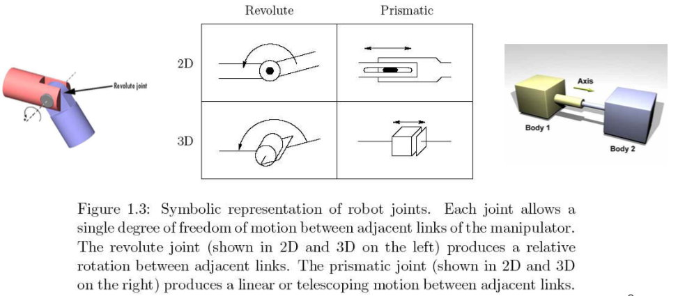
Robot manipulators are composed of links connected by joints into a kinematic chain. Two joint types cover almost every industrial manipulator:
- Revolute joint: allows relative rotation between two links.
- Prismatic joint: allows a linear relative motion between two links.
Degrees of Freedom
The number of joints determines the degrees of freedom (DOF) of the manipulator. A typical manipulator should possess at least six independent DOF: three for positioning and three for orientation. With fewer than six DOF the arm cannot reach every point in its work environment with an arbitrary orientation.
Workspace
The workspace is the total volume swept out by the end-effector as the manipulator executes all possible motions. It is usually described in two parts:
- Reachable workspace: the entire set of points reachable by the manipulator.
- Dexterous workspace: the subset of the reachable workspace that the manipulator can reach with an arbitrary orientation of the end-effector.
Common Kinematic Arrangements
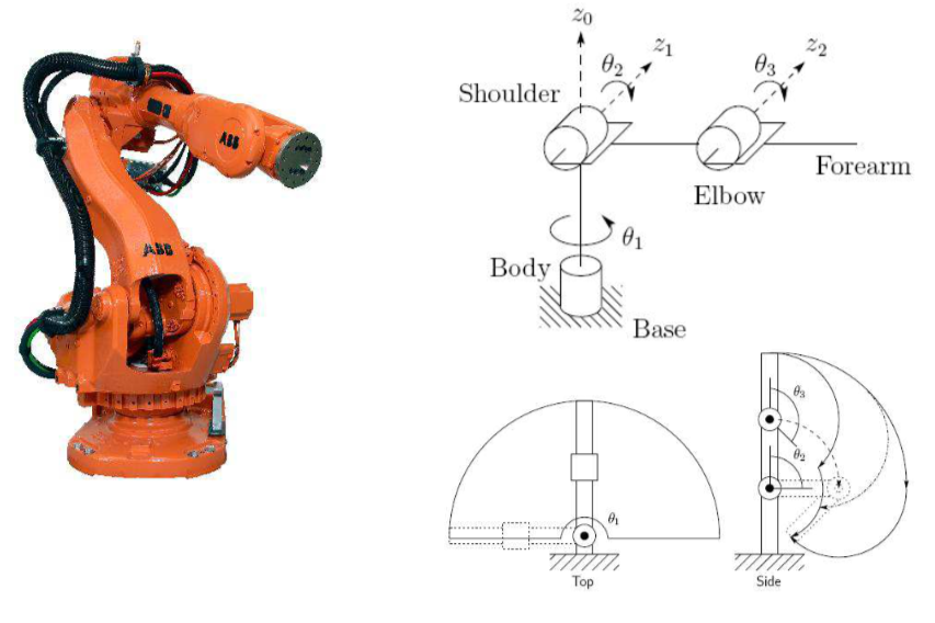
Articulated configuration (RRR)
This configuration provides relatively large freedom of movement in a compact space. Its links and joints are analogous to the human arm.
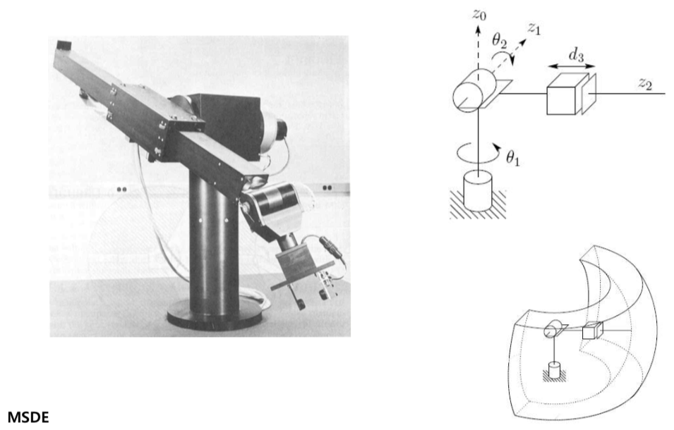
Spherical configuration (RRP)
The third joint of the articulated robot is replaced by a prismatic joint. The Stanford arm is an example of a spherical manipulator.
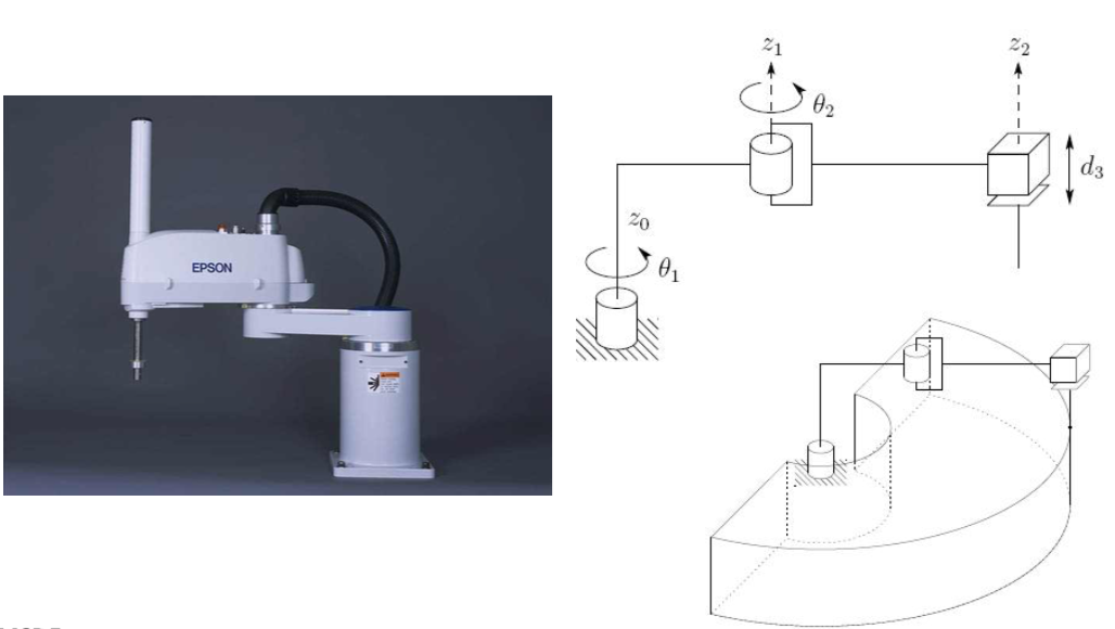
SCARA configuration (RRP)
The SCARA (Selective Compliant Articulated Robot for Assembly) has $z_0$, $z_1$ and $z_2$ parallel. It is ideal for table-top assembly such as pick-and-place tasks.
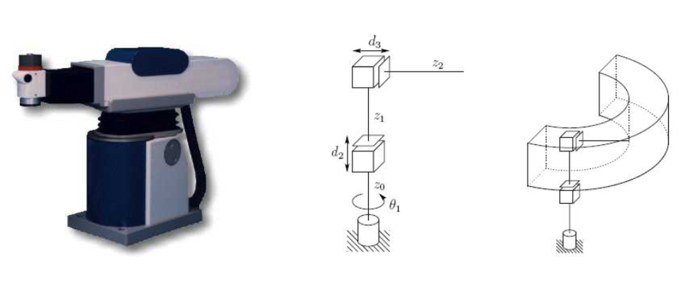
Cylindrical configuration (RPP)
The first joint is revolute, while the second and third joints are prismatic. This arrangement is often used in materials-transfer tasks.
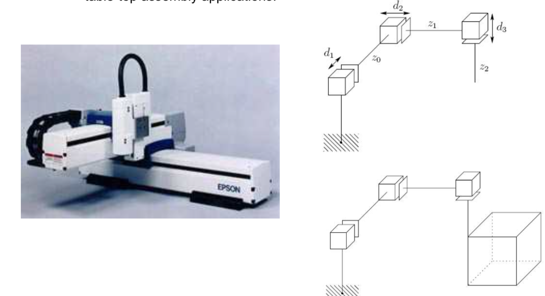
Cartesian configuration (PPP)
This configuration is useful for table-top assembly applications and is often used in pick-and-place operations.
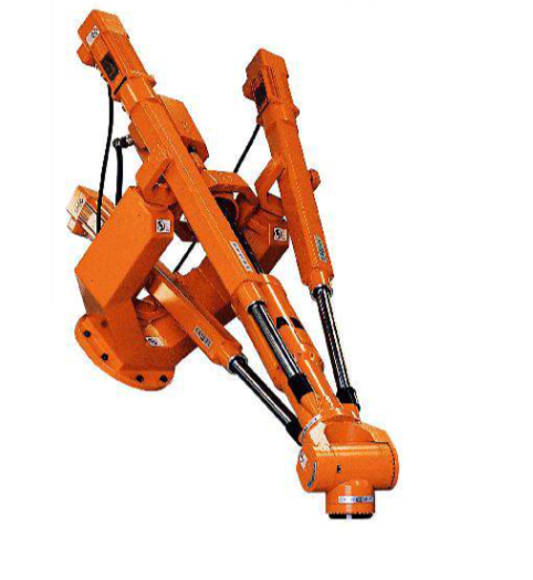
Parallel manipulator
A parallel manipulator forms a closed chain by using several independent kinematic chains connecting the base to the end-effector. The closed chain results in greater structural rigidity, so these robots are generally much more rigid than serial-link robots.
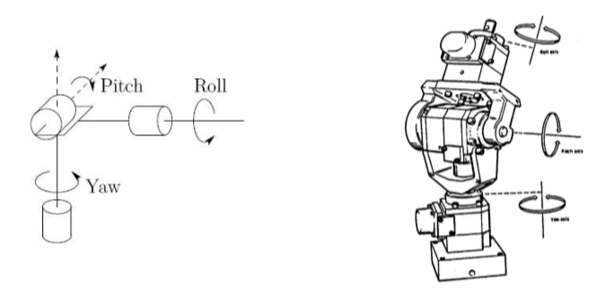
Wrists and End-Effectors
The wrist of a manipulator refers to the joints in the kinematic chain between the arm and the hand. It is increasingly common to design manipulators with a spherical wrist, meaning a wrist whose three joint axes intersect at a common point. A six-DOF arm is then split as three DOF for the arm plus three DOF for the wrist: the arm and wrist assemblies are used primarily to position and orient the end-effector (the hand). The simplest end-effectors are grippers.
Problem 1: Forward Kinematics
The first problem is to describe the position and orientation of the tool, that is, to determine the position and orientation of the end-effector in terms of the joint variables (angles or displacements).
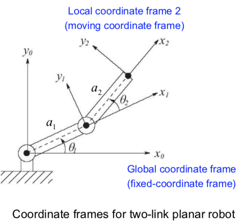
Forward kinematic equations
Tool (end-effector) position
$$ \begin{aligned} x &= a_1 \cos\theta_1 + a_2 \cos(\theta_1 + \theta_2) \\ y &= a_1 \sin\theta_1 + a_2 \sin(\theta_1 + \theta_2) \end{aligned} $$Tool (end-effector) orientation
The orientation is captured by the rotation matrix
$$ \begin{bmatrix} i_2 \cdot i_0 & j_2 \cdot i_0 \\ i_2 \cdot j_0 & j_2 \cdot j_0 \end{bmatrix} = \begin{bmatrix} \cos(\theta_1 + \theta_2) & -\sin(\theta_1 + \theta_2) \\ \sin(\theta_1 + \theta_2) & \cos(\theta_1 + \theta_2) \end{bmatrix} $$Note: the Denavit-Hartenberg convention and the homogeneous transformation are needed to express this relationship systematically.
Problem 2: Inverse Kinematics
In order to command the robot to move to an arbitrary position, we need the joint variables in terms of the $x$ and $y$ coordinates, so the forward kinematic equations are normally needed in advance.
Since the forward kinematic equations are nonlinear, a solution may not be easy to obtain, and there may be many solutions or an infinite number of solutions. In that case we can impose additional constraints to select one.
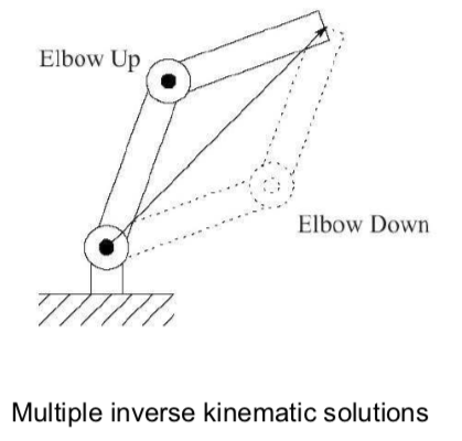
Law of Cosines
$$ \begin{aligned} \cos\theta_2 &= \frac{x^2 + y^2 - a_1^2 - a_2^2}{2 a_1 a_2} \triangleq D \\ \therefore\ \theta_2 &= \cos^{-1}(D) \end{aligned} $$This is not the best approach, because $\cos^{-1}$ cannot distinguish between the elbow-up and elbow-down configurations. Using the sine as well removes the ambiguity:
$$ \begin{aligned} \sin^2\theta_2 + \cos^2\theta_2 &= 1 \;\rightarrow\; \sin\theta_2 = \pm\sqrt{1 - D^2} \\ \therefore\ \theta_2 &= \operatorname{atan2}\!\left(\pm\sqrt{1 - D^2},\; D\right) \end{aligned} $$The sign determines the elbow-up and elbow-down solutions.
Inverse kinematic equations
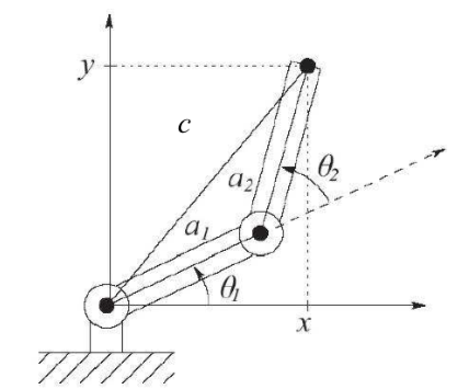
The result can be verified by substituting it back into the forward kinematics (a cross-check).
Another way - Closed form
In the closed form approach, $\theta_1$ and $\theta_2$ are expressed in terms of $x$ and $y$ using the forward kinematics. Squaring $x$ and $y$ and adding them eliminates $\theta_1$, which yields $\cos\theta_2$ and $\sin\theta_2$ and hence $\theta_2$.
$$ \begin{aligned} x &= a_1 \cos\theta_1 + a_2 \cos(\theta_1 + \theta_2) \\ y &= a_1 \sin\theta_1 + a_2 \sin(\theta_1 + \theta_2) \\ &\qquad\qquad \triangledown \\[4pt] x^2 &= a_1^2 \cos^2\theta_1 + a_2^2 \cos^2(\theta_1 + \theta_2) + 2 a_1 a_2 \cos\theta_1 \cos(\theta_1 + \theta_2) \\ &= a_1^2 \cos^2\theta_1 + a_2^2 \cos^2(\theta_1 + \theta_2) + a_1 a_2 \left[\cos(2\theta_1 + \theta_2) + \cos\theta_2\right] \\ y^2 &= a_1^2 \sin^2\theta_1 + a_2^2 \sin^2(\theta_1 + \theta_2) + 2 a_1 a_2 \sin\theta_1 \sin(\theta_1 + \theta_2) \\ &= a_1^2 \sin^2\theta_1 + a_2^2 \sin^2(\theta_1 + \theta_2) - a_1 a_2 \left[\cos(2\theta_1 + \theta_2) - \cos\theta_2\right] \\ &\qquad\qquad \triangledown \\[4pt] x^2 + y^2 &= a_1^2 + a_2^2 + 2 a_1 a_2 \cos\theta_2 \\ &\qquad\qquad \triangledown \\[4pt] \cos\theta_2 &= \frac{x^2 + y^2 - a_1^2 - a_2^2}{2 a_1 a_2} \triangleq D \\ \sin\theta_2 &= \pm\sqrt{1 - D^2} \\[4pt] \therefore\ \theta_2 &= \operatorname{atan2}\!\left(\pm\sqrt{1 - D^2},\; D\right) \end{aligned} $$To recover $\theta_1$, multiply the $x$ equation by $\cos\theta_1$ and the $y$ equation by $\sin\theta_1$, then add them to obtain Equation (1). Next multiply the $x$ equation by $\sin\theta_1$ and the $y$ equation by $\cos\theta_1$, then subtract them to obtain Equation (2). Combining (1) and (2) with $x$ and $y$ by addition and subtraction isolates $\cos\theta_1$ and $\sin\theta_1$, and hence $\theta_1$.
$$ \begin{aligned} x &= a_1 \cos\theta_1 + a_2 \cos(\theta_1 + \theta_2) \\ y &= a_1 \sin\theta_1 + a_2 \sin(\theta_1 + \theta_2) \\[4pt] x \cos\theta_1 &= a_1 \cos^2\theta_1 + a_2 \cos\theta_1 \left(\cos\theta_1 \cos\theta_2 - \sin\theta_1 \sin\theta_2\right) \\ y \sin\theta_1 &= a_1 \sin^2\theta_1 + a_2 \sin\theta_1 \left(\sin\theta_1 \cos\theta_2 + \cos\theta_1 \sin\theta_2\right) \\ &\qquad\qquad \triangledown \\ x \cos\theta_1 + y \sin\theta_1 &= a_1 + a_2 \cos\theta_2 \qquad (1) \\[8pt] x \sin\theta_1 &= a_1 \sin\theta_1 \cos\theta_1 + a_2 \sin\theta_1 \left(\cos\theta_1 \cos\theta_2 - \sin\theta_1 \sin\theta_2\right) \\ y \cos\theta_1 &= a_1 \sin\theta_1 \cos\theta_1 + a_2 \cos\theta_1 \left(\sin\theta_1 \cos\theta_2 + \cos\theta_1 \sin\theta_2\right) \\ &\qquad\qquad \triangledown \\ x \sin\theta_1 - y \cos\theta_1 &= -a_2 \sin\theta_2 \qquad (2) \\[8pt] (x^2 + y^2)\cos\theta_1 &= x\left(a_1 + a_2 \cos\theta_2\right) + y\, a_2 \sin\theta_2 \qquad \because x \cdot (1) - y \cdot (2) \\ &\qquad\qquad \triangledown \\ \cos\theta_1 &= \frac{x\left(a_1 + a_2 \cos\theta_2\right) + y\, a_2 \sin\theta_2}{x^2 + y^2} \\[8pt] (x^2 + y^2)\sin\theta_1 &= y\left(a_1 + a_2 \cos\theta_2\right) - x\, a_2 \sin\theta_2 \qquad \because y \cdot (1) + x \cdot (2) \\ &\qquad\qquad \triangledown \\ \sin\theta_1 &= \frac{y\left(a_1 + a_2 \cos\theta_2\right) - x\, a_2 \sin\theta_2}{x^2 + y^2} \\[8pt] \therefore\ \theta_1 &= \operatorname{atan2}\!\left(y\left(a_1 + a_2 \cos\theta_2\right) - x\, a_2 \sin\theta_2,\; x\left(a_1 + a_2 \cos\theta_2\right) + y\, a_2 \sin\theta_2\right) \end{aligned} $$Another way - Numerical Solution
In contrast to the closed form (geometric) solution, the numerical solution absolutely requires the forward kinematics.
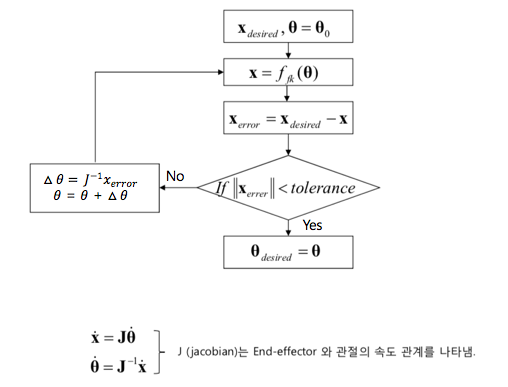
Problem 3: Velocity Kinematics
In order to follow a contour at constant velocity, or at any prescribed velocity, we must know the relationship between the velocity of the tool (end-effector) and the joint velocities. Differentiating the forward kinematic equations gives
$$ \begin{aligned} \dot{x} &= -a_1 \dot{\theta}_1 \sin\theta_1 - a_2 \left(\dot{\theta}_1 + \dot{\theta}_2\right)\sin(\theta_1 + \theta_2) \\ \dot{y} &= a_1 \dot{\theta}_1 \cos\theta_1 + a_2 \left(\dot{\theta}_1 + \dot{\theta}_2\right)\cos(\theta_1 + \theta_2) \end{aligned} $$With $\mathbf{x} = \begin{bmatrix} x & y \end{bmatrix}^{T}$ and $\boldsymbol{\theta} = \begin{bmatrix} \theta_1 & \theta_2 \end{bmatrix}^{T}$, this becomes
$$ \begin{aligned} \dot{\mathbf{x}} &= J \dot{\boldsymbol{\theta}} \\ &= \begin{bmatrix} \dfrac{\partial x}{\partial \theta_1} & \dfrac{\partial x}{\partial \theta_2} \\[6pt] \dfrac{\partial y}{\partial \theta_1} & \dfrac{\partial y}{\partial \theta_2} \end{bmatrix} \begin{bmatrix} \dot{\theta}_1 \\ \dot{\theta}_2 \end{bmatrix} \\ &= \begin{bmatrix} -a_1 \sin\theta_1 - a_2 \sin(\theta_1 + \theta_2) & -a_2 \sin(\theta_1 + \theta_2) \\ a_1 \cos\theta_1 + a_2 \cos(\theta_1 + \theta_2) & a_2 \cos(\theta_1 + \theta_2) \end{bmatrix} \begin{bmatrix} \dot{\theta}_1 \\ \dot{\theta}_2 \end{bmatrix} \end{aligned} $$where $J$ is the Jacobian. Using the inverse Jacobian gives
$$ \begin{aligned} \dot{\boldsymbol{\theta}} &= J^{-1} \dot{\mathbf{x}} \\ \begin{bmatrix} \dot{\theta}_1 \\ \dot{\theta}_2 \end{bmatrix} &= \frac{1}{a_1 a_2 \sin\theta_2} \begin{bmatrix} a_2 \cos(\theta_1 + \theta_2) & a_2 \sin(\theta_1 + \theta_2) \\ -a_1 \cos\theta_1 - a_2 \cos(\theta_1 + \theta_2) & -a_1 \sin\theta_1 - a_2 \sin(\theta_1 + \theta_2) \end{bmatrix} \begin{bmatrix} \dot{x} \\ \dot{y} \end{bmatrix} \end{aligned} $$A singular configuration is one in which no inverse Jacobian exists. At a singular configuration the manipulator cannot move in certain directions:
$$ \begin{aligned} \det J &= a_1 a_2 \sin\theta_2 = 0 \\ \therefore\ \theta_2 &= 0 \quad \text{or} \quad \pi \end{aligned} $$Problem 4: Path Planning and Trajectory Generation
Path planning
Path planning determines a path in task space that moves the robot to a goal position while avoiding collisions with objects in its workspace, without time considerations — that is, without considering velocities and accelerations.
Trajectory Generation
Trajectory generation determines the time history of the manipulator along a given path.
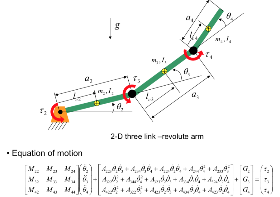
Problem 5: Dynamics
Dynamics describes the relationship between motion and forces (the equation of motion) and answers the question of how much force is required to achieve a given motion. Rigid body dynamics treats a target object that undergoes no strain or deformation:
$$ M(q)\,\ddot{q} + C(q, \dot{q})\,\dot{q} + G(q) = \tau $$- $M$: inertia matrix.
- $C$: centrifugal and Coriolis matrix.
- $G$: gravity matrix.
- $q$: generalized coordinate (angle or position).
- $\tau$: generalized force (torque or force).
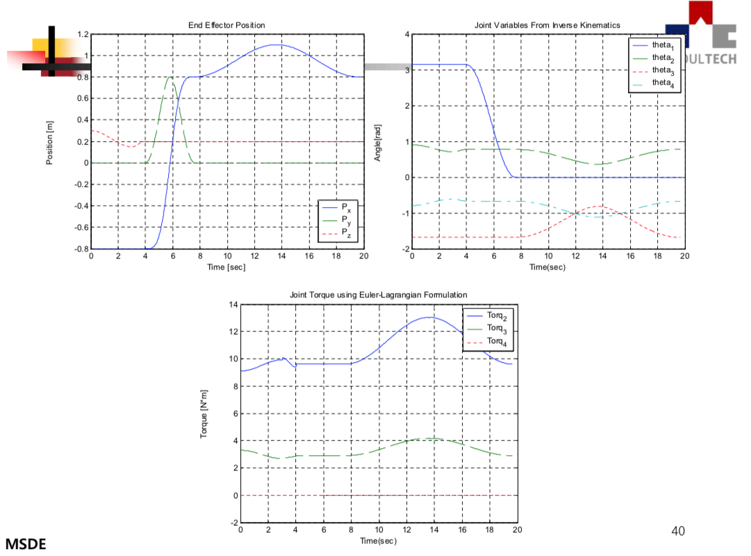
Inverse dynamics computes the required joint torques or forces that lead to a given robot motion, whereas forward dynamics computes the robot motion resulting from the applied joint torques or forces.
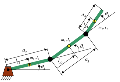
Example 1: Three link-revolute arm
Problem 6: Position Control
The control problem for a robot manipulator is the problem of determining the time history of the joint inputs (joint forces, torques, or actuator inputs such as voltage) required to cause the end-effector to execute a desired motion.
There are many control techniques and methodologies, and the appropriate one depends on the hardware, software and application:
- Cartesian manipulator vs. elbow-type manipulator.
- DC motor with reduction gear vs. high-torque DC motor without gear (high-end designs for interaction).
- Point-to-point path vs. continuous path.
The more complicated the hardware, the more advanced the control method that is required.
Example: Independent Joint Position Control
This is the simplest type of control strategy. Each axis is controlled as a SISO (single-input/single-output) system, and any coupling effects due to the motion of the other links are either ignored or treated as a disturbance. The objectives are tracking and disturbance rejection.
The moment — and therefore the disturbance — varies with the pose, but it is neglected here because of the high gear ratio.
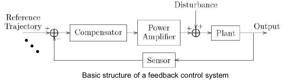
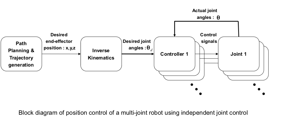
Each joint has to follow the desired joint angle accurately.
Problem 7: Force Control
Why force control? Pure position control is not adequate for tasks that involve extensive contact with the environment, such as assembly, grinding and deburring. In such tasks the force must be controlled as well, because a slight deviation of the end-effector would cause it either to lose contact or to press too strongly. Hybrid control (position plus force control) addresses this: a force control strategy is one that modifies position trajectories based on the sensed forces.
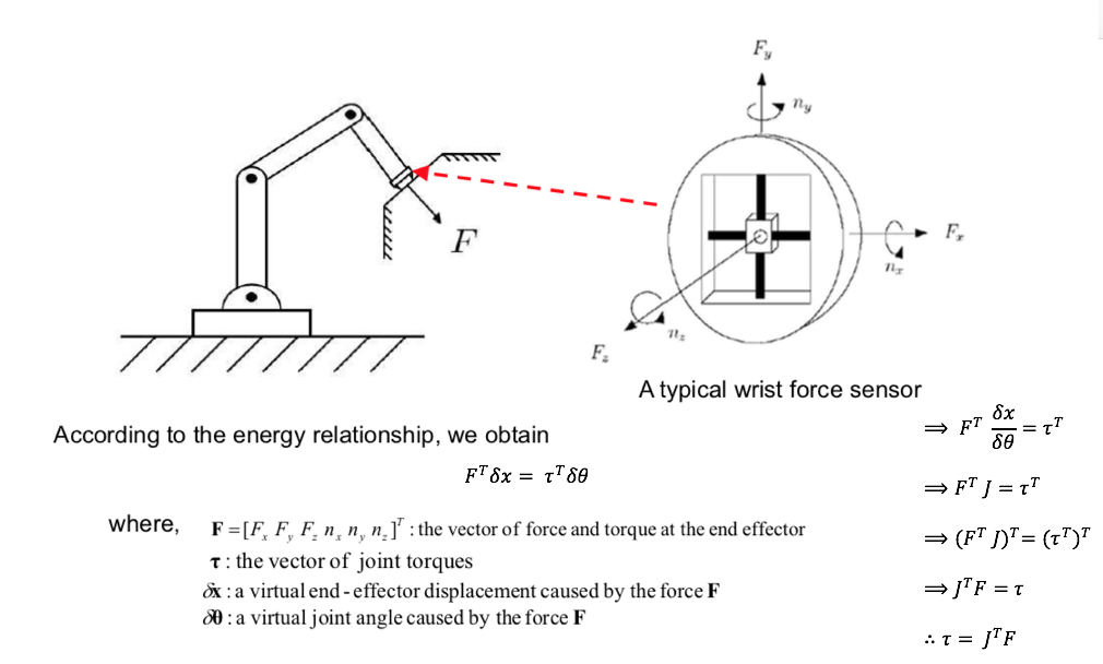
The end-effector forces are related to the joint torques.