Robot Dynamics & Control: Lecture 4 - Inverse Kinematics

Introduction

This chapter is concerned with the inverse problem of finding the joint variables in terms of the end-effector position and orientation. After formulating the general inverse kinematics (I.K.) problem, we study the principle of kinematic decoupling, which simplifies the I.K. problem by separating position from orientation. We then describe a geometric approach for solving the position problem, while exploiting the Euler angle parameterization to solve the orientation problem.

$$ \begin{bmatrix} \theta_1 \\ \vdots \\ \theta_n \\ d_1 \\ \vdots \\ d_n \end{bmatrix} = f(x, y, z, \psi, \theta, \phi) $$

The General I.K. Problem

Given a desired pose

$$ H(x, y, z, \psi, \theta, \phi) = \begin{bmatrix} R & o \\ 0 & 1 \end{bmatrix} \in SE(3) $$

with $R \in SO(3)$, find one or all solutions of the equation

$$ T^0_n(q_1, \cdots, q_n) = H $$

where

$$ T^0_n(q_1, \cdots, q_n) = A_1(q_1) \cdots A_n(q_n) $$

Our task is to find the values of the joint variables $q_1, \ldots, q_n$ such that $T^0_n(q_1, \ldots, q_n) = H$.

$$ \begin{aligned} T^0_n(q_1, \cdots, q_n) &= H \\ \begin{bmatrix} T_{11} & T_{12} & T_{13} & T_{14} \\ T_{21} & T_{22} & T_{23} & T_{24} \\ T_{31} & T_{32} & T_{33} & T_{34} \\ T_{41} & T_{42} & T_{43} & T_{44} \end{bmatrix} &= \begin{bmatrix} c_{\phi}c_{\theta} & -s_{\phi}c_{\psi} + c_{\phi}s_{\theta}s_{\psi} & s_{\phi}s_{\psi} + c_{\phi}s_{\theta}c_{\psi} & x \\ s_{\phi}c_{\theta} & c_{\phi}c_{\psi} + s_{\phi}s_{\theta}s_{\psi} & -c_{\phi}s_{\psi} + s_{\phi}s_{\theta}c_{\psi} & y \\ -s_{\theta} & c_{\theta}s_{\psi} & c_{\theta}c_{\psi} & z \\ 0 & 0 & 0 & 1 \end{bmatrix} \end{aligned} $$

The given matrix $H$ therefore combines a roll/pitch/yaw rotation with respect to the inertial frame and a translation with respect to the inertial frame — equivalently, a translation followed by a roll/pitch/yaw rotation with respect to the current frame.

The above equation results in 12 nonlinear equations in $n$ unknown variables, which can be written as

$$ T_{ij}(q_1, \cdots, q_n) = h_{ij}, \qquad i = 1, 2, 3, \quad j = 1, \ldots, 4 $$

where $T_{ij}$ and $h_{ij}$ refer to the 12 nontrivial entries of $T^0_n$ and $H$.

Example

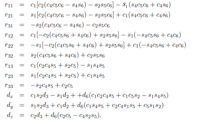
Recall the Stanford manipulator. Suppose that the desired position and orientation of the final frame are given by

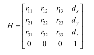
To find the corresponding variables $\theta_1, \ldots, \theta_6$ we must solve the following simultaneous set of nonlinear trigonometric equations:

Note
It is too difficult to solve this directly in closed form.
Therefore it is necessary to develop efficient and systematic techniques.
The inverse kinematics problem may or may not have a solution.
Even if a solution exists, it may or may not be unique.

There are two families of inverse kinematics solutions:

A closed form solution
A numerical solution

A closed form solution means an explicit relationship of the form

$$ q_k = f_k(h_{11}, \ldots, h_{34}), \qquad k = 1, \ldots, n $$

Closed form solutions have two advantages. First, they are more accurate and faster than numerical solutions. Second, they allow one to develop rules for choosing a particular solution among several: the desired pose can be selected by choosing a sign, which a numerical method cannot do.

Kinematic Decoupling

For manipulators having six joints with the last three joint axes intersecting at a point, it is possible to decouple the I.K. problem into two simpler problems:

Inverse position kinematics
Inverse orientation kinematics

Let us suppose that there are exactly six degrees of freedom and that the last three joint axes intersect at a point $o_c$:

$$ \begin{aligned} R^0_6(q_1, \ldots, q_6) &= R \\ o^0_6(q_1, \ldots, q_6) &= o \end{aligned} $$

$o$ and $R$ are the desired position and orientation of the tool frame with respect to the world coordinate system.

We assume that the axes $z_3$, $z_4$ and $z_5$ intersect at $o_c$, and hence that the origins $o_3$, $o_4$ and $o_5$ lie at the wrist center $o_c$. Motion of the final three links about these axes will not change the position of $o_c$. Thus the position of the wrist center is a function of only the first three joint variables ($\theta_1$, $\theta_2$ and $d_3$).

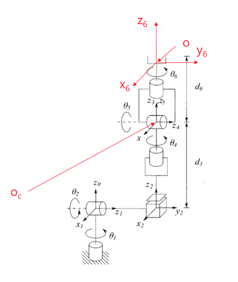
The origin of the tool frame, $o$, is then

$$ \begin{aligned} o &= o^0_c + R^0_5 \begin{bmatrix} 0 \\ 0 \\ d_6 \end{bmatrix} \\ \rightarrow \quad o^0_c &= o - R^0_5 \begin{bmatrix} 0 \\ 0 \\ d_6 \end{bmatrix} \\ \rightarrow \quad o^0_c &= o - R \begin{bmatrix} 0 \\ 0 \\ d_6 \end{bmatrix} \end{aligned} $$

The third columns of $R^0_6$ and $R^0_5$ are the same.

$$ \begin{bmatrix} x_c \\ y_c \\ z_c \end{bmatrix} = \begin{bmatrix} o_x - d_6 r_{13} \\ o_y - d_6 r_{23} \\ o_z - d_6 r_{33} \end{bmatrix} \quad \text{where} \quad R = \begin{bmatrix} r_{11} & r_{12} & r_{13} \\ r_{21} & r_{22} & r_{23} \\ r_{31} & r_{32} & r_{33} \end{bmatrix} $$

Using the above equation we may find the values of the first three joint variables.
This determines the orientation transformation $R^0_3$, which depends only on those first three joint variables.

The orientation of the end-effector relative to the frame $o_3 x_3 y_3 z_3$ is then

$$ \begin{aligned} R &= R^0_6 = R^0_3 R^3_6 \\[6pt] R^3_6 &= \left(R^0_3\right)^{-1} R = \left(R^0_3\right)^T R \end{aligned} $$

Here $R$ is given, $R^0_3$ can be calculated once the first three joint variables are known, and $R^3_6$ is the unknown.

The final three joint variables can then be found as a set of Euler angles corresponding to $R^3_6$.

For this class of manipulators the determination of the inverse kinematics can be summarized by the following algorithm.

Step 1. Find $q_1, q_2, q_3$ such that the wrist center $o_c$ has coordinates given by

$$ o^0_c = o - R^0_5 \begin{bmatrix} 0 \\ 0 \\ d_6 \end{bmatrix} = o - R \begin{bmatrix} 0 \\ 0 \\ d_6 \end{bmatrix} $$

Step 2. Using the joint variables determined in Step 1, evaluate $R^0_3$.

Step 3. Find a set of Euler angles corresponding to the rotation matrix

$$ R^3_6 = \left(R^0_3\right)^{-1} R = \left(R^0_3\right)^T R $$

Inverse Position: A Geometric Approach

We can use a geometric approach to find the variables $q_1, q_2, q_3$ corresponding to $o^0_c$. There are two reasons for preferring the geometric approach: most manipulator designs are kinematically simple (without joint offsets), usually consisting of one of the five basic configurations with a spherical wrist; and there are few techniques that can handle the general I.K. problem for arbitrary configurations.

The general idea of the geometric approach is to solve for the joint variable $q_i$ by projecting the manipulator onto the $x_{i-1} - y_{i-1}$ plane and solving a simple trigonometry problem.

Articulated Configuration

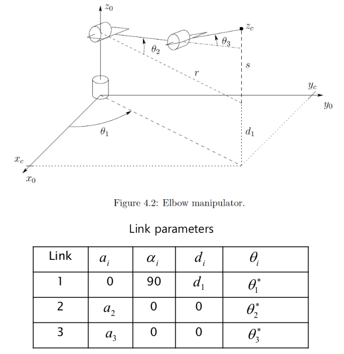
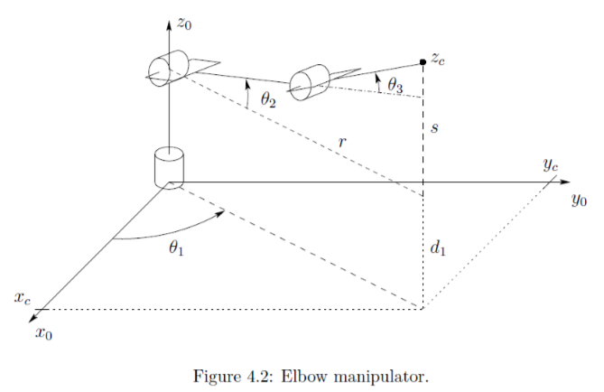
Consider the elbow manipulator shown in Fig. 4.2, with the components of $o^0_c$ denoted by $x_c, y_c, z_c$. We project $o_c$ onto the $x_0 - y_0$ plane.

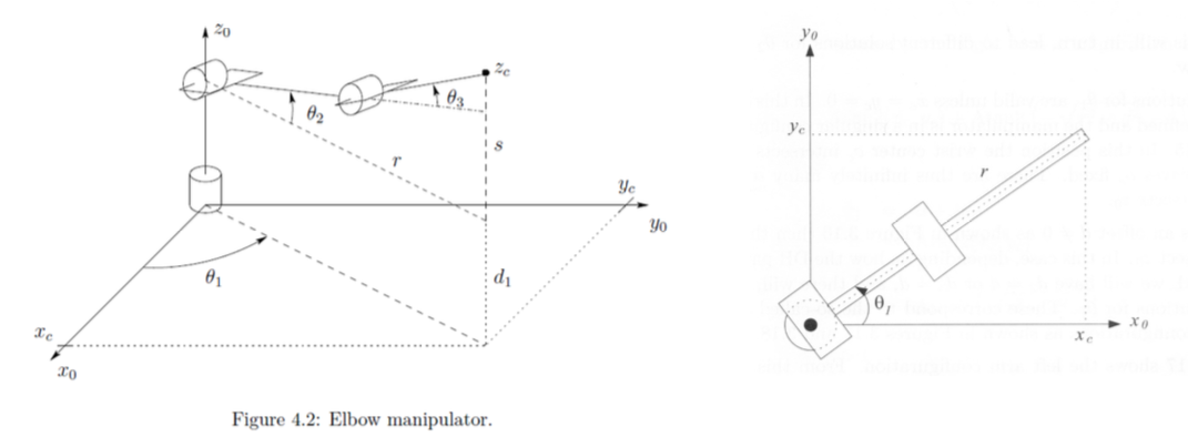
From this projection,

$$ \theta_1 = \operatorname{atan2}(y_c,\, x_c) $$

Note that a second valid solution for $\theta_1$ is

$$ \theta_1 = \pi + \operatorname{atan2}(y_c,\, x_c) $$

This second solution leads to different solutions for $\theta_2$ and $\theta_3$.

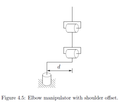
The above solution is valid unless $x_c = y_c = 0$. In that case the manipulator is in a singular configuration, as shown in Fig. 4.5, and there are infinitely many solutions for $\theta_1$.

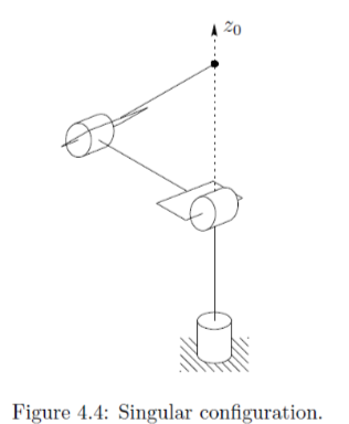
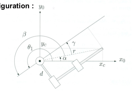
If there is an offset $d$, then the wrist center cannot intersect $z_0$. In this case there are only two solutions for $\theta_1$, which correspond to the so-called left arm and right arm configurations.

Case 1: left arm configuration

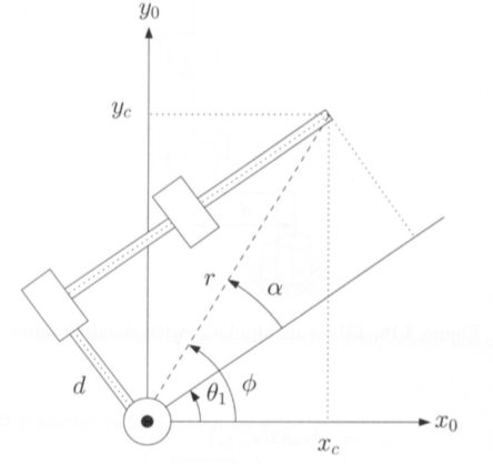
Geometrically,

$$ \begin{aligned} \theta_1 &= \phi - \alpha \\ \text{where } \phi &= \operatorname{atan2}(y_c,\, x_c), \\ \alpha &= \operatorname{atan2}\!\left(d,\; \sqrt{r^2 - d^2}\right) = \operatorname{atan2}\!\left(d,\; \sqrt{x^2_c + y^2_c - d^2}\right) \end{aligned} $$

Case 2: right arm configuration

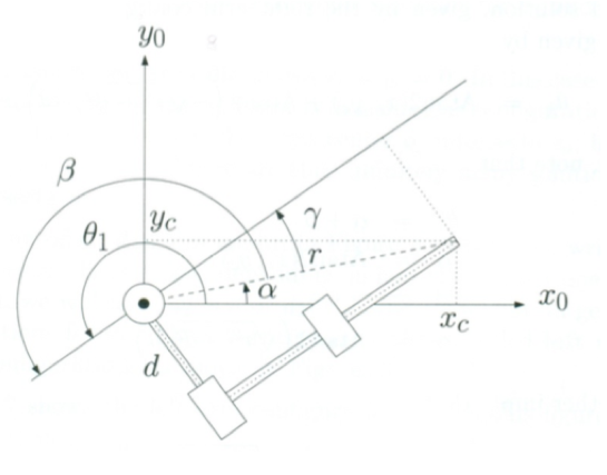
Geometrically,

$$ \begin{aligned} \theta_1 &= \alpha + \beta \\ \text{where } \alpha &= \operatorname{atan2}(y_c,\, x_c), \\ \beta &= \gamma + \pi = \operatorname{atan2}\!\left(d,\; \sqrt{r^2 - d^2}\right) + \pi = \operatorname{atan2}\!\left(-d,\; -\sqrt{r^2 - d^2}\right) \end{aligned} $$

To find the angles $\theta_2$ and $\theta_3$ for the elbow manipulator given $\theta_1$, we consider the plane formed by the second and third links.

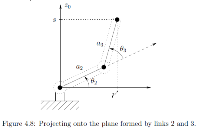
As before,

$$ \begin{aligned} \theta_3 &= \operatorname{atan2}\!\left(\pm\sqrt{1 - D^2},\; D\right) \\ \text{where } D &= \cos\theta_3 = \frac{r'^2 + s^2 - a^2_2 - a^2_3}{2 a_2 a_3} = \frac{\left(x^2_c + y^2_c - d^2\right) + \left(z_c - d_1\right)^2 - a^2_2 - a^2_3}{2 a_2 a_3} \end{aligned} $$

Similarly,

$$ \begin{aligned} \theta_2 &= \operatorname{atan2}(s,\, r') - \operatorname{atan2}\!\left(a_3 s_3,\; a_2 + a_3 c_3\right) \\ &= \operatorname{atan2}\!\left(z_c - d_1,\; \sqrt{x^2_c + y^2_c - d^2}\right) - \operatorname{atan2}\!\left(a_3 s_3,\; a_2 + a_3 c_3\right) \end{aligned} $$

The two solutions for $\theta_3$ correspond to the elbow-up and elbow-down positions, respectively.

Spherical Configuration

We now solve the inverse position kinematics for a three-DOF spherical manipulator. The first joint variable is the base rotation, and its solution is

$$ \theta_1 = \operatorname{atan2}(y_c,\, x_c) \qquad x_c \neq 0 \ \text{ or } \ y_c \neq 0 $$

The second solution is

$$ \theta_1 = \pi + \operatorname{atan2}(y_c,\, x_c) $$

If both $x_c$ and $y_c$ are zero, the configuration is singular and $\theta_1$ may take on any value.

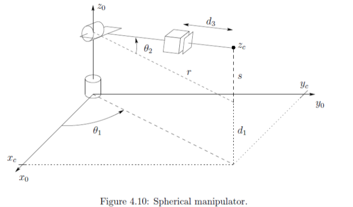
The angle $\theta_2$ is given by

$$ \theta_2 = \operatorname{atan2}(s,\, r) $$

where $r^2 = x^2_c + y^2_c$ and $s = z_c - d_1$. The linear distance $d_3$ is found as

$$ d_3 = \sqrt{r^2 + s^2} = \sqrt{x^2_c + y^2_c + \left(z_c - d_1\right)^2} $$

There are two solutions to the inverse position kinematics as long as the wrist center does not intersect $z_0$ (that is, $x_c, y_c \neq 0$).
If there is an offset, then there will be left arm and right arm configurations.

Inverse Orientation

The inverse position problem gives the values of the first three joint variables corresponding to a given position of the wrist center. The inverse orientation problem is that of finding the values of the final three joint variables corresponding to a given orientation with respect to the frame $o_3 x_3 y_3 z_3$; it can be interpreted as the problem of finding a set of Euler angles corresponding to a given rotation matrix $R$.

Recall that the rotation matrix obtained for the spherical wrist has the same form as the rotation matrix for the Euler transformation:

$$ \begin{aligned} T^3_6 = A_4 A_5 A_6 &= \begin{bmatrix} R^3_6 & o^3_6 \\ 0 & 1 \end{bmatrix} \\ &= \begin{bmatrix} c_4 c_5 c_6 - s_4 s_6 & -c_4 c_5 s_6 - s_4 c_6 & c_4 s_5 & c_4 s_5 d_6 \\ s_4 c_5 c_6 + c_4 s_6 & -s_4 c_5 s_6 + c_4 c_6 & s_4 s_5 & s_4 s_5 d_6 \\ -s_5 c_6 & s_5 s_6 & c_5 & c_5 d_6 \\ 0 & 0 & 0 & 1 \end{bmatrix} \end{aligned} $$ $$ \begin{aligned} R_{z,\phi} R_{y,\theta} R_{z,\psi} &= \begin{bmatrix} c_{\phi} & -s_{\phi} & 0 \\ s_{\phi} & c_{\phi} & 0 \\ 0 & 0 & 1 \end{bmatrix} \begin{bmatrix} c_{\theta} & 0 & s_{\theta} \\ 0 & 1 & 0 \\ -s_{\theta} & 0 & c_{\theta} \end{bmatrix} \begin{bmatrix} c_{\psi} & -s_{\psi} & 0 \\ s_{\psi} & c_{\psi} & 0 \\ 0 & 0 & 1 \end{bmatrix} \\ &= \begin{bmatrix} c_{\phi}c_{\theta}c_{\psi} - s_{\phi}s_{\psi} & -c_{\phi}c_{\theta}s_{\psi} - s_{\phi}c_{\psi} & c_{\phi}s_{\theta} \\ s_{\phi}c_{\theta}c_{\psi} + c_{\phi}s_{\psi} & -s_{\phi}c_{\theta}s_{\psi} + c_{\phi}c_{\psi} & s_{\phi}s_{\theta} \\ -s_{\theta}c_{\psi} & s_{\theta}s_{\psi} & c_{\theta} \end{bmatrix} \end{aligned} $$

Comparing the two gives

$$ \begin{aligned} \theta_4 &= \phi \\ \theta_5 &= \theta \\ \theta_6 &= \psi \end{aligned} $$

Even though they have different forms, the joint angles are easy to find.

Example 1: Articulated Manipulator with Spherical Wrist

Using the D-H parameters we can derive the matrix $R^0_3$:

$$ R^0_3 = \begin{bmatrix} c_1 c_{23} & -c_1 s_{23} & s_1 \\ s_1 c_{23} & -s_1 s_{23} & -c_1 \\ s_{23} & c_{23} & 0 \end{bmatrix} $$

The matrix $R^3_6$ is the upper-left $3 \times 3$ submatrix of the matrix product $A_4 A_5 A_6$, given by

$$ R^3_6 = \begin{bmatrix} c_4 c_5 c_6 - s_4 s_6 & -c_4 c_5 s_6 - s_4 c_6 & c_4 s_5 \\ s_4 c_5 c_6 + c_4 s_6 & -s_4 c_5 s_6 + c_4 c_6 & s_4 s_5 \\ -s_5 c_6 & s_5 s_6 & c_5 \end{bmatrix} $$

The equation to be solved for the final three variables, with $R$ given, is therefore

$$ \begin{aligned} R^3_6 &= \left(R^0_3\right)^T R \\ \therefore \begin{bmatrix} c_4 c_5 c_6 - s_4 s_6 & -c_4 c_5 s_6 - s_4 c_6 & c_4 s_5 \\ s_4 c_5 c_6 + c_4 s_6 & -s_4 c_5 s_6 + c_4 c_6 & s_4 s_5 \\ -s_5 c_6 & s_5 s_6 & c_5 \end{bmatrix} &= \begin{bmatrix} c_1 c_{23} & s_1 c_{23} & s_{23} \\ -c_1 s_{23} & -s_1 s_{23} & c_{23} \\ s_1 & -c_1 & 0 \end{bmatrix} \begin{bmatrix} r_{11} & r_{12} & r_{13} \\ r_{21} & r_{22} & r_{23} \\ r_{31} & r_{32} & r_{33} \end{bmatrix} \end{aligned} $$

Comparing the third column,

$$ \begin{aligned} c_4 s_5 &= c_1 c_{23} r_{13} + s_1 c_{23} r_{23} + s_{23} r_{33} \\ s_4 s_5 &= -c_1 s_{23} r_{13} - s_1 s_{23} r_{23} + c_{23} r_{33} \\ c_5 &= s_1 r_{13} - c_1 r_{23} \\ \therefore\ \theta_5 &= \operatorname{atan2}\!\left(\pm\sqrt{1 - \left(s_1 r_{13} - c_1 r_{23}\right)^2},\; s_1 r_{13} - c_1 r_{23}\right) \end{aligned} $$

If the positive square root is chosen,

$$ \begin{aligned} \theta_4 &= \operatorname{atan2}\!\left(s_4 s_5,\; c_4 s_5\right) \\ &= \operatorname{atan2}\!\left(-c_1 s_{23} r_{13} - s_1 s_{23} r_{23} + c_{23} r_{33},\; c_1 c_{23} r_{13} + s_1 c_{23} r_{23} + s_{23} r_{33}\right) \end{aligned} $$

Comparing the third row,

$$ \begin{aligned} -s_5 c_6 &= s_1 r_{11} - c_1 r_{21} \\ s_5 s_6 &= s_1 r_{12} - c_1 r_{22} \\ \theta_6 &= \operatorname{atan2}\!\left(s_5 s_6,\; -\left(-s_5 c_6\right)\right) \\ \therefore\ \theta_6 &= \operatorname{atan2}\!\left(s_1 r_{12} - c_1 r_{22},\; -s_1 r_{11} + c_1 r_{21}\right) \end{aligned} $$

If the negative square root is chosen,

$$ \begin{aligned} \theta_4 &= \operatorname{atan2}\!\left(-s_4 s_5,\; -c_4 s_5\right) \\ &= \operatorname{atan2}\!\left(c_1 s_{23} r_{13} + s_1 s_{23} r_{23} - c_{23} r_{33},\; -c_1 c_{23} r_{13} - s_1 c_{23} r_{23} - s_{23} r_{33}\right) \\[6pt] \theta_6 &= \operatorname{atan2}\!\left(-s_5 s_6,\; -s_5 c_6\right) \\ &= \operatorname{atan2}\!\left(-s_1 r_{12} + c_1 r_{22},\; s_1 r_{11} - c_1 r_{21}\right) \end{aligned} $$

If $s_5 = 0$, then the joint axes $z_3$ and $z_5$ are collinear. This is a singular configuration, so there are infinitely many solutions and only the sum $\theta_4 + \theta_6$ can be determined.

Example 2: Complete Solution for the Elbow Manipulator

This is one complete inverse kinematic solution of the six-DOF elbow manipulator, which has no joint offsets and a spherical wrist.

Given the end-effector position $o$ and orientation $R$,

$$ o = \begin{bmatrix} o_x \\ o_y \\ o_z \end{bmatrix}, \qquad R = \begin{bmatrix} r_{11} & r_{12} & r_{13} \\ r_{21} & r_{22} & r_{23} \\ r_{31} & r_{32} & r_{33} \end{bmatrix} $$

the wrist center and the joint variables are

$$ \begin{aligned} x_c &= o_x - d_6 r_{13} \\ y_c &= o_y - d_6 r_{23} \\ z_c &= o_z - d_6 r_{33} \\[6pt] \theta_1 &= \operatorname{atan2}(y_c,\, x_c) \\ \theta_2 &= \operatorname{atan2}\!\left(z_c - d_1,\; \sqrt{x^2_c + y^2_c}\right) - \operatorname{atan2}\!\left(a_3 s_3,\; a_2 + a_3 c_3\right) \\ \theta_3 &= \operatorname{atan2}\!\left(\pm\sqrt{1 - D^2},\; D\right), \quad \text{where } D = \frac{x^2_c + y^2_c + \left(z_c - d_1\right)^2 - a^2_2 - a^2_3}{2 a_2 a_3} \\ \theta_4 &= \operatorname{atan2}\!\left(\pm\left(-c_1 s_{23} r_{13} - s_1 s_{23} r_{23} + c_{23} r_{33}\right),\; \pm\left(c_1 c_{23} r_{13} + s_1 c_{23} r_{23} + s_{23} r_{33}\right)\right) \\ \theta_5 &= \operatorname{atan2}\!\left(\pm\sqrt{1 - \left(s_1 r_{13} - c_1 r_{23}\right)^2},\; s_1 r_{13} - c_1 r_{23}\right) \\ \theta_6 &= \operatorname{atan2}\!\left(\pm\left(s_1 r_{12} - c_1 r_{22}\right),\; \pm\left(-s_1 r_{11} + c_1 r_{21}\right)\right) \end{aligned} $$

Example 3: SCARA Manipulator

The forward kinematics is defined by

There is no solution of the above equation unless $R$ is of the form

$$ R = \begin{bmatrix} c_{\alpha} & s_{\alpha} & 0 \\ s_{\alpha} & -c_{\alpha} & 0 \\ 0 & 0 & -1 \end{bmatrix} $$

If this is the case, the sum $\theta_1 + \theta_2 - \theta_4$ is determined by

$$ \theta_1 + \theta_2 - \theta_4 = \alpha = \operatorname{atan2}(r_{12},\, r_{11}) $$

Projecting the manipulator configuration onto the $x_0 - y_0$ plane gives

$$ \begin{aligned} \theta_2 &= \operatorname{atan2}\!\left(\pm\sqrt{1 - c^2_2},\; c_2\right), \quad \text{where } c_2 = \frac{x^2_c + y^2_c - a^2_1 - a^2_2}{2 a_1 a_2} \\ \theta_1 &= \operatorname{atan2}(y_c,\, x_c) - \operatorname{atan2}\!\left(a_2 s_2,\; a_1 + a_2 c_2\right) \end{aligned} $$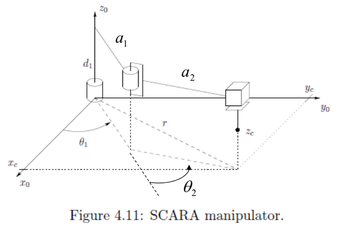

Then

$$ \begin{aligned} \theta_4 &= \theta_1 + \theta_2 - \alpha \\ &= \theta_1 + \theta_2 - \operatorname{atan2}(r_{12},\, r_{11}) \end{aligned} $$

and finally

$$ d_3 = -o_z - d_4 $$

Inverse Kinematics: A Numerical Approach

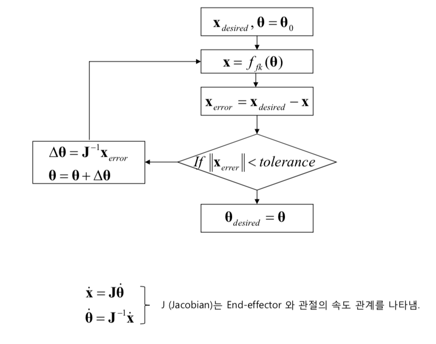
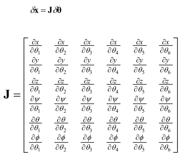
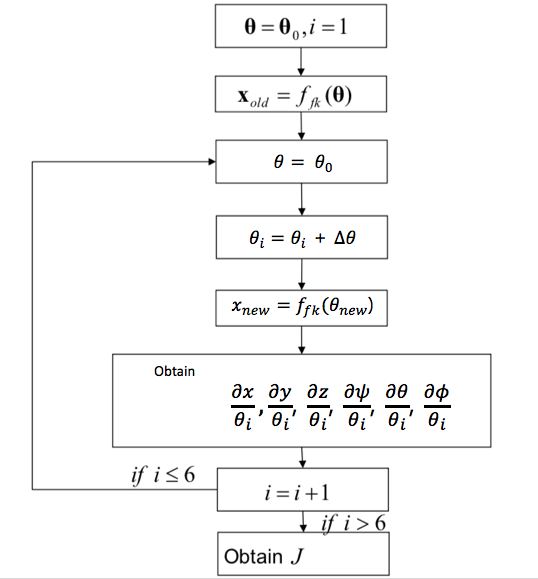
The basic flowchart is as follows.