Model-based-augmented model-free RL (Dyna-Q, I2A)

Dyna-Q

Once a model of the environment is learned, it is possible to augment MF algorithms with MB transitions. The MF algorithm (e.g. Q-learning) learns from transitions \((s, a, r, s')\) sampled either with:

1. real experience: online interaction with the environment.
2. simulated experience: simulated transitions by the model.

Figure 1: Dyna-Q alternates between online updates and simulated “offline” updates from the model.

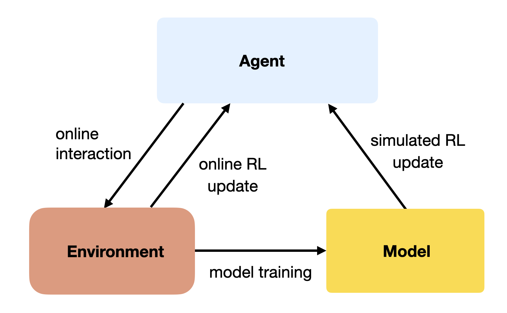
If the simulated transitions are realistic enough, the MF algorithm can converge using much less real transitions, thereby reducing its sample complexity.

The Dyna-Q algorithm [@Sutton1990] is an extension of Q-learning to integrate a model \(M(s, a) = (s', r')\). It alternates between online updates of the agent using the real environment and (possible multiple) offline updates using the model.

Dyna-Q [@Sutton1990]

• Initialize values \(Q(s, a)\) and model \(M(s, a)\).

• for \(t \in [0, T_\text{total}]\):

  • Select \(a_t\) using \(Q\), take it on the real environment and observe \(s_{t+1}\) and \(r_{t+1}\).

  • Update the Q-value of the real action:

  \[\Delta Q(s_t, a_t) = \alpha \, (r_{t+1} + \gamma \, \max_a Q(s_{t+1}, a) - Q(s_t, a_t))\]

  • Update the model:

  \[M(s_t, a_t) \leftarrow (s_{t+1}, r_{t+1})\]

  • for \(K\) steps:

    • Sample a state \(s_k\) from a list of visited states.

    • Select \(a_k\) using \(Q\), predict \(s_{k+1}\) and \(r_{k+1}\) using the model \(M(s_k, a_k)\).

    • Update the Q-value of the imagined action:

    \[\Delta Q(s_k, a_k) = \alpha \, (r_{k+1} + \gamma \, \max_a Q(s_{k+1}, a) - Q(s_k, a_k))\]

It is interesting to notice that Dyna-Q is the inspiration for DQN and its experience replay memory. In DQN, the ERM stores real transitions generated in the past and recovers them later intact, while in Dyna-Q, the model generates imagined transitions approximated based on past real transitions. Interleaving on-policy and off-policy updates is also the core idea of ACER (section ?@sec-acer).

I2A - Imagination-augmented agents

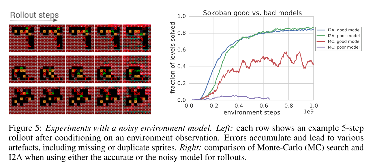
I2A [@Weber2017] is a model-based augmented model-free method: it trains a MF algorithm (A3C) with the help of rollouts generated by a MB model. The authors showcase their algorithm on the puzzle environment Sokoban, where you need to move boxes to specified locations.

Figure 2: Game of Sokoban used to showcase the abilities of I2A. Source: @Weber2017

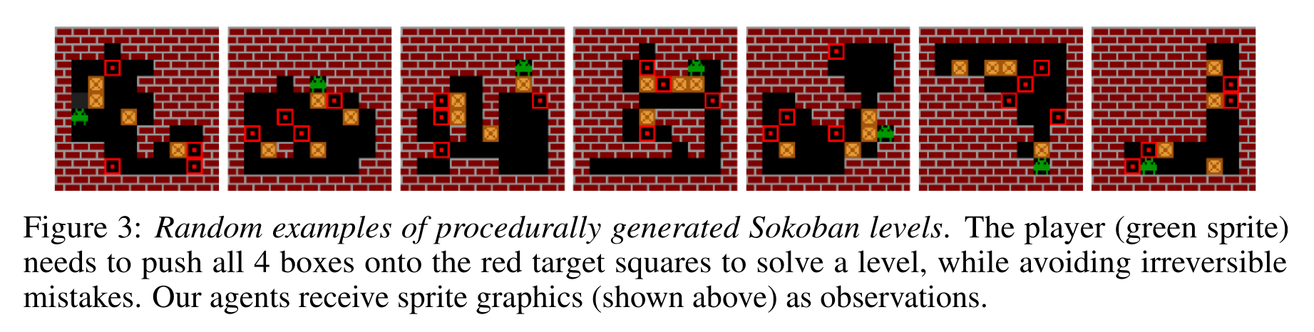
Sokoban is a quite hard game, as actions are irreversible (you can get stuck) and the solution requires many actions (sparse rewards). MF methods are bad at this game as they learn through trials-and-(many)-errors.

I2A is composed of several different modules. We will now have a look at them one by one.

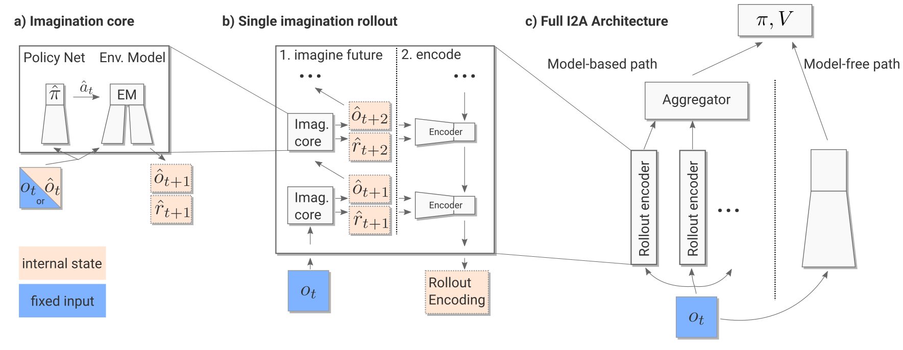
Environment model

Figure 3: Environment model of I2A. Source: @Weber2017

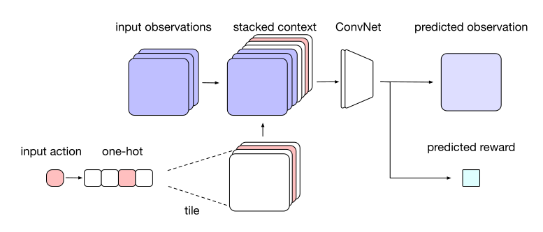
The environment model learns to predict the next frame and the next reward based on the four last frames and the chosen action:

\[ (o_{t-3}, o_{t-2}, o_{t-1}, o_{t}, a_t) \rightarrow (o_{t+1}, r_{t+1}) \]

As Sokoban is a POMDP (partially observable), the notation uses observations \(o_t\) instead of states \(s_t\), but it does not really matter here.

The neural network is a sort of convolutional autoencoder, taking additionally an action \(a\) as input and predicting the next reward. Formally, the output “image” being different from the input, the neural network is not an autoencoder but belongs to the family of segmentation networks such as SegNet [@Badrinarayanan2016] or U-net [@Ronneberger2015]. It can be pretrained using a random policy, and later fine-tuned during training.

Imagination core

Figure 4: Imagination core. Source: @Weber2017

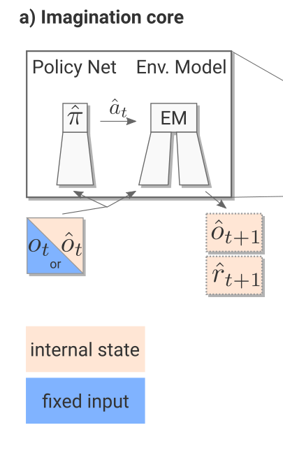
The imagination core is composed of the environment model \(M(s, a)\) and a rollout policy \(\hat{\pi}\). The rollout policy \(\hat{\pi}\) is a simple and fast policy. It does not have to be the trained policy \(\pi\): It could even be a random policy, or a pretrained policy using for example A3C directly. In I2A, the rollout policy \(\hat{\pi}\) is obtained through policy distillation of the bigger policy network \(\pi\).

Policy distillation [@Rusu2016]

The small rollout policy network \(\hat{\pi}\) tries to copy the outputs \(\pi(s, a)\) of the whole model. This is a supervised learning task: we just need minimize the KL divergence between the two policies:

\[\mathcal{L}(\hat{\theta}) = \mathbb{E}_{s, a} [D_\text{KL}(\hat{\pi}(s, a) || \pi(s, a))]\]

As the network is smaller, it won’t be quite as good as \(\pi\) (although not dramatically), but its learning objective is simpler: supervised learning is much easier than RL, especially when the rewards are sparse. A very small network (up to 90% of the original parameters) is often enough for the same functionality.

Figure 5: Policy distillation. The student model learns to imitate the teacher model through supervised learning, which is much easier than RL.

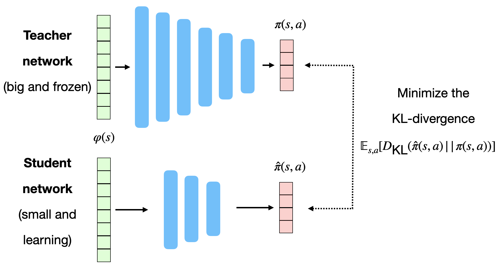
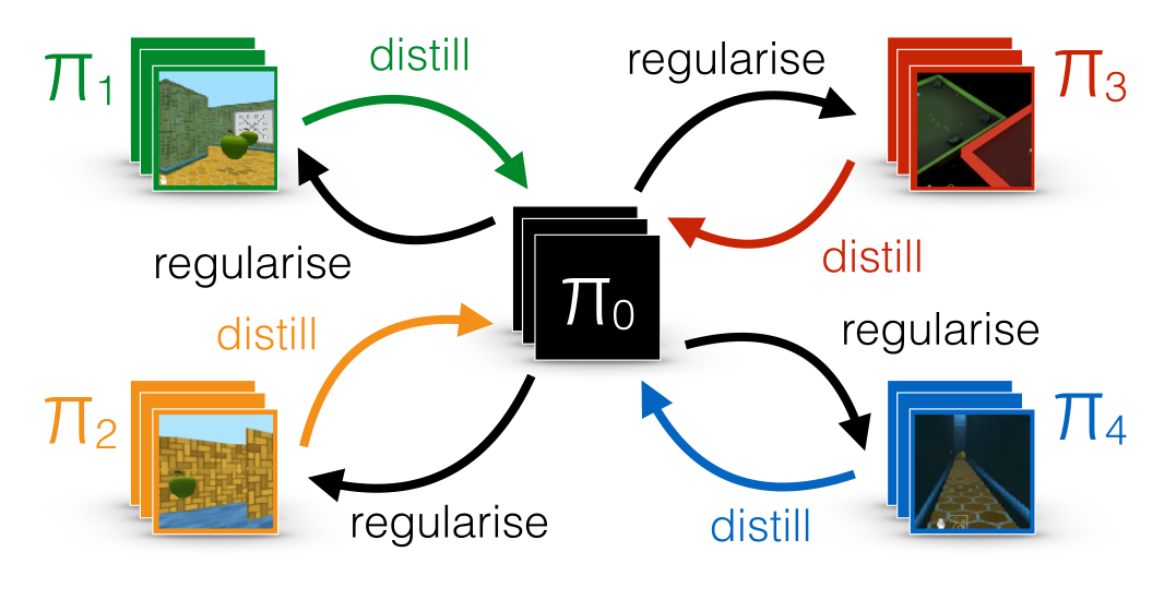
In general, policy distillation can be used to ensure generalization over different environments, as in Distral [@Teh2017]. Each learning algorithms learns its own task, but tries not to diverge too much from a shared policy, which turns out to be good at all tasks.

Figure 6: Distral architecture. Each sub-policy \(\pi_i\) learns a specific environment. The central policy \(\pi_0\) distills knowledge from the sub-policies, while forcing them through regularization not to diverge too much. Ultimately, the central policy becomes able to solve all the environments. Source: @Teh2017

Imagination rollout module

Figure 7: Imagination rollout module. Source: @Weber2017

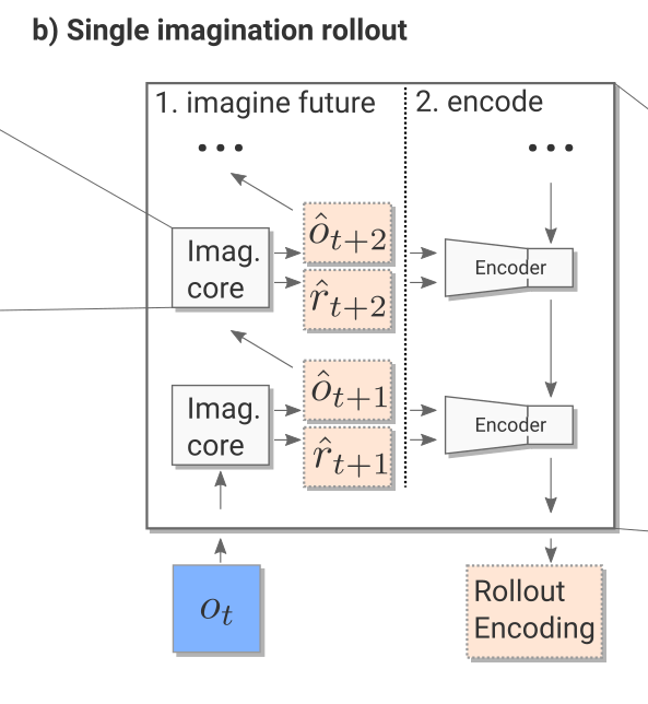
The imagination rollout module uses the imagination core to predict iteratively the next \(\tau\) frames and rewards using the current frame \(o_t\) and the rollout policy:

\[(o_{t-3}, o_{t-2}, o_{t-1}, o_{t}) \rightarrow \hat{o}_{t+1} \rightarrow \hat{o}_{t+2} \rightarrow \ldots \rightarrow \hat{o}_{t+\tau}\]

The \(\tau\) frames and rewards are passed backwards to a convolutional LSTM (from \(t+\tau\) to \(t\)) which produces an embedding / encoding of the rollout. The output of the imagination rollout module is a vector \(e_i\) (the final state of the LSTM) representing the whole rollout, including the (virtually) obtained rewards. Note that because of the stochasticity of the rollout policy \(\hat{\pi}\), different rollouts can lead to different encoding vectors.

Model-free path

Figure 8: Model-free path Source: @Weber2017

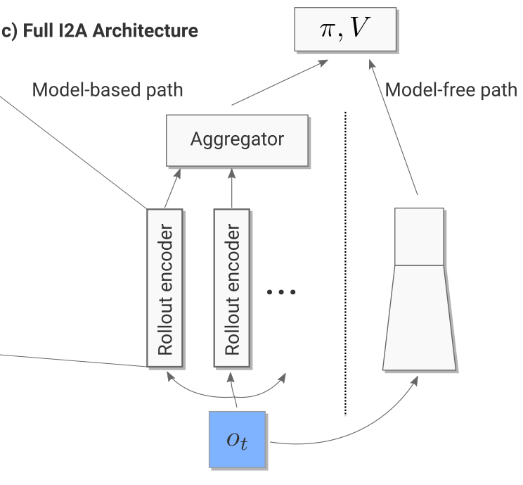
For the current observation \(o_t\) (and the three frames before), we then generate one rollout per possible action (5 in Sokoban):

• What would happen if I do action 1?
• What would happen if I do action 2?
• etc.

The resulting vectors are concatenated to the output of model-free path (a convolutional neural network taking the current observation as input).

Full model

Altogether, we have a huge NN with weights \(\theta\) (model, rollout encoder, MF path) between the input observation \(o_t\) and the output policy \(\pi\) (plus the critic \(V\)).

Figure 9: Complete architecture of I2A. Source: @Weber2017

We can then learn the policy \(\pi\) and value function \(V\) using the n-step advantage actor-critic (A3C) :

\[\nabla_\theta \mathcal{J}(\theta) = \mathbb{E}_{s_t \sim \rho_\theta, a_t \sim \pi_\theta}[\nabla_\theta \log \pi_\theta (s_t, a_t) \, (\sum_{k=0}^{n-1} \gamma^{k} \, r_{t+k+1} + \gamma^n \, V_\varphi(s_{t+n}) - V_\varphi(s_t)) ]\]

\[\mathcal{L}(\varphi) = \mathbb{E}_{s_t \sim \rho_\theta, a_t \sim \pi_\theta}[(\sum_{k=0}^{n-1} \gamma^{k} \, r_{t+k+1} + \gamma^n \, V_\varphi(s_{t+n}) - V_\varphi(s_t))^2]\]

The complete architecture may seem complex, but everything is differentiable so we can apply backpropagation and train the network end-to-end using multiple workers. It is simply the A3C algorithm (MF), but augmented by MB rollouts, i.e. with explicit information about the (emulated) future.

Results

Unsurprisingly, I2A performs better than A3C on Sokoban. The deeper the rollout, the better:

Figure 10: Performance of I2A. Source: @Weber2017

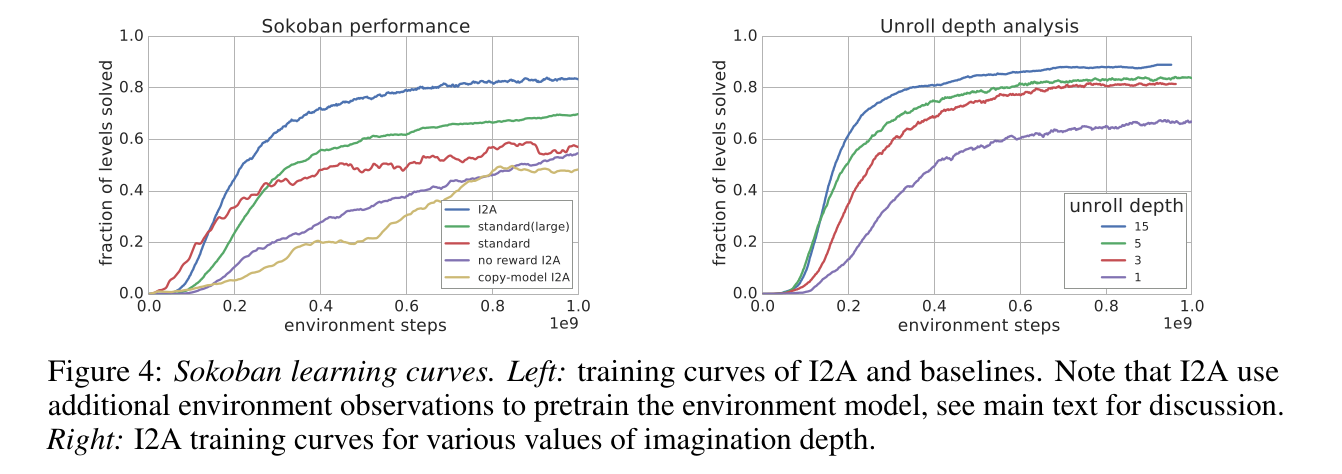
The model does not even have to be perfect: the MF path can compensate for imperfections:

Figure 11: Influence of noise. Source: @Weber2017